ScopeSim Sources
ScopeSim Source and SourceField Overview
What is a Source?
Source is the top-level target container passed into OpticalTrain.observe(). It combines:
Spatial information: where light is on sky (
source.fields)Spectral information: what spectrum each component has (
source.spectra)Metadata: extra context (
source.meta)
A single Source can hold multiple components (e.g., stars + diffuse background + cube).
What is a SourceField?
Source.fields is a list that stores SourceField objects representing one spatial/spectral component.
Available field types (subclasses of SourceField):
``TableSourceField``
Stores an
astropy.table.Tablewith point-source rows.Typical columns:
x,y,ref,weight.refmaps each row to an entry insource.spectra.
``ImageSourceField``
Stores a 2D
fits.ImageHDU(surface-brightness map).Uses WCS in header for sky-to-pixel mapping.
Usually linked to one spectrum via header metadata (e.g.,
SPEC_REF).
``CubeSourceField``
Stores a 3D cube (
fits.ImageHDU) with spatial + wavelength axes.Contains its own spectral axis (not just one average spectrum).
[1]:
import matplotlib.pyplot as plt
import numpy as np
import astropy.units as u
from astropy.table import Table, vstack
from astropy.io import fits

import scopesim_templates as sim_tp
from scopesim.source.source import Source
from scopesim.source.source_fields import TableSourceField, ImageSourceField, CubeSourceField
import scopesim.source.source_templates  as source_templates
import scopesim.source.source_utils as source_utils

def plot_source(source):
    wave = np.linspace(0.3, 2.5, 1001) * u.um
    num_fields = len(source.fields)
    fig, axs = plt.subplots(figsize=(6,2*num_fields), nrows=num_fields, ncols=2, width_ratios=[1,2], constrained_layout=True)
    if num_fields == 1:
        axs = np.array([axs])
    for i, field in enumerate(source.fields):
        ax1, ax2 = axs[i]
        ax1.imshow(field.data, origin='lower', cmap='viridis')
        ax2.plot(wave, field.spectrum(wave))
        ax1.set_title('Spatial Profile')
        ax1.set_xlabel('X (arcsec)')
        ax1.set_ylabel('Y (arcsec)')
        ax2.set_title('Spectrum')
        ax2.set_xlabel('Wavelength (um)')
        ax2.set_ylabel(r'Flux (ph s$^{-1}$ cm$^{-2}$ $\AA^{-1}$)')
/Users/yashvi/Desktop/ZShooter/.venv/lib/python3.12/site-packages/tqdm/auto.py:21: TqdmWarning: IProgress not found. Please update jupyter and ipywidgets. See https://ipywidgets.readthedocs.io/en/stable/user_install.html
  from .autonotebook import tqdm as notebook_tqdm
How to create Source objects
A) From a point-source table + spectra
[2]:
tbl = Table(
    data=[[0.0, 1.2], [0.0, -0.5], [0, 0], [1.0, 0.7]],
    names=["x", "y", "ref", "weight"],
)
tbl["x"].unit = u.arcsec
tbl["y"].unit = u.arcsec

ps = Source(table=tbl, spectra=[source_templates.vega_spectrum(10)])
ps.fields
[2]:
[TableSourceField(field=<Table length=2>
    x       y     ref   weight
  arcsec  arcsec
 float64 float64 int64 float64
 ------- ------- ----- -------
     0.0     0.0     0     1.0
     1.2    -0.5     0     0.7, spectra={0: <synphot.spectrum.SourceSpectrum object at 0x11205ee10>})]
B) From an image HDU + spectrum
[3]:
img = np.ones((64, 64), dtype=float)
hdr = fits.Header(cards={'CUNIT1':'arcsec', 'CUNIT2':'arcsec', 'CDELT1':1, 'CDELT2':1}) # need to include this minimal header
hdu = fits.ImageHDU(data=img, header=hdr)
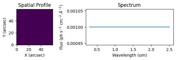
im = Source(image_hdu=hdu, spectra=[source_templates.ab_spectrum(mag=20)]) # ab_spectrum creates a spectrum with constant flux in magnitude space of given mag (which does not mean constant in erg/s/cm2/Angstrom)
print(im.fields)
plot_source(im)
[ImageSourceField(field=<astropy.io.fits.hdu.image.ImageHDU object at 0x1139d55b0>, wcs=WCS Keywords

Number of WCS axes: 2
CTYPE : '' ''
CUNIT : 'deg' 'deg'
CRVAL : 0.0 0.0
CRPIX : 0.0 0.0
PC1_1 PC1_2  : 1.0 0.0
PC2_1 PC2_2  : 0.0 1.0
CDELT : 0.000277777777777777 0.000277777777777777
NAXIS : 64  64, spectra={0: <synphot.spectrum.SourceSpectrum object at 0x10de474a0>})]

NOTE: Can also use src.source_templates.uniform_source() to create the above source in one step as shown below. The default spatial sampling is 1 arcsec/pixel.
[4]:
im2 = source_templates.uniform_source(source_templates.ab_spectrum(mag=20), extent=64)
print(im2.fields)
plot_source(im2)
[ImageSourceField(field=<astropy.io.fits.hdu.image.ImageHDU object at 0x113cbc830>, wcs=WCS Keywords

Number of WCS axes: 2
CTYPE : 'RA---TAN' 'DEC--TAN'
CUNIT : 'deg' 'deg'
CRVAL : 0.0 0.0
CRPIX : 32.5 32.5
PC1_1 PC1_2  : 1.0 0.0
PC2_1 PC2_2  : 0.0 1.0
CDELT : -0.00027777777777778 0.00027777777777778
NAXIS : 64  64, spectra={0: <synphot.spectrum.SourceSpectrum object at 0x113acede0>})]

To create a uniform source in PHOTLAM units (photons/s/cm^2/Angstrom), use ConstFlux1D with the appropriate amplitude (e.g., 0.001 for 1 photon/s/cm^2/Angstrom):
[5]:
sp = source_templates.ConstFlux1D(amplitude=0.001) # synphot model, default unit is photon/s/cm^2/Angstrom
waves = np.geomspace(100, 300000, 50000)
lookup = sp(waves)
im3 = source_templates.uniform_source(
                                    source_templates.SourceSpectrum(source_templates.Empirical1D, points=waves, lookup_table=lookup),  # synphot spectrum
                                    extent=60)
plot_source(im3)
C) From helper templates (quick start) available in scopesim_templates package
[6]:
# star
star = sim_tp.star(filter_name='V', amplitude=10*u.ABmag) # spectra taken from 'spextra' package
star.plot()
[6]:
<Axes: xlabel='x [arcsec]', ylabel='y [arcsec]'>

[7]:
# Galaxy
gal = sim_tp.extragalactic.galaxies.spiral_two_component(extent=200*u.arcsec, fluxes=(15, 15)*u.mag)  # loaded from saved fits template of NGC1232L
gal.shift(dy=-30*0.004)
plot_source(gal)

Other available galaxy models include galaxy, galaxy3d, and elliptical. See scopesim_templates.extragalactic.galaxies for details.
Useful sources
A uniform source to simulate dome flats
[8]:
# Let's say we want a high-power halogen bulb emitting a 3000 K blackbody spectrum, uniformly illuminating a 1 arcmin x 1 arcmin area on the sky. We can create this source as follows:
domeflat = sim_tp.calibration.flat_field(temperature=3000*u.K, amplitude=4*u.ABmag, filter_curve='V', extend=60)
plot_source(domeflat)

Arc lamps for wavelength calibration
[9]:
# load line list
uvb = Table.read('line_lists/ThAr_XSHOOTER_UVB_lines.dat', delimiter='|', format='ascii', header_start=0)
neir = Table.read('line_lists/Ne_IR_MOSFIRE_lines.dat', delimiter='|', format='ascii', header_start=0)
arir = Table.read('line_lists/Ar_IR_MOSFIRE_lines.dat', delimiter='|', format='ascii', header_start=0)
lines = vstack([uvb, neir, arir])
lines
[9]:
| col0 | wave | ion | NIST | Instr | amplitude | Source | _1 |
|---|---|---|---|---|---|---|---|
| int64 | float64 | str4 | int64 | int64 | float64 | str20 | int64 |
| -- | 3094.261313368305 | ThAr | 1 | 32 | 218.70677052723238 | wavemodel.py | -- |
| -- | 3140.0171522371547 | ThAr | 1 | 32 | 148.12281124090538 | wavemodel.py | -- |
| -- | 3170.5540268969266 | ThAr | 1 | 32 | 158.8138285062605 | wavemodel.py | -- |
| -- | 3181.1243070684113 | ThAr | 1 | 32 | 227.88057703827917 | wavemodel.py | -- |
| -- | 3189.181869102448 | ThAr | 1 | 32 | 222.56046465150408 | wavemodel.py | -- |
| -- | 3233.222527087156 | ThAr | 1 | 32 | 199.46752294459446 | wavemodel.py | -- |
| -- | 3239.0583334075486 | ThAr | 1 | 32 | 145.47867955933862 | wavemodel.py | -- |
| -- | 3244.661251438086 | ThAr | 1 | 32 | 208.4018341765855 | wavemodel.py | -- |
| -- | 3245.1958097699485 | ThAr | 1 | 32 | 253.38302082586046 | wavemodel.py | -- |
| ... | ... | ... | ... | ... | ... | ... | ... |
| -- | 22118.66 | ArI | 1 | 32 | 360.0 | keck_mosfire_webpage | -- |
| -- | 22539.74 | ArI | 1 | 32 | 40.0 | keck_mosfire_webpage | -- |
| -- | 22978.37 | ArI | 1 | 32 | 150.0 | keck_mosfire_webpage | -- |
| -- | 23139.52 | ArI | 1 | 32 | 11910.0 | keck_mosfire_webpage | -- |
| -- | 23851.54 | ArI | 1 | 32 | 10480.0 | keck_mosfire_webpage | -- |
| -- | 23973.06 | ArI | 1 | 32 | 13070.0 | keck_mosfire_webpage | -- |
| -- | 24783.37 | ArI | 1 | 32 | 150.0 | keck_mosfire_webpage | -- |
| -- | 25132.13 | ArI | 1 | 32 | 5760.0 | keck_mosfire_webpage | -- |
| -- | 25512.18 | ArI | 1 | 32 | 3750.0 | keck_mosfire_webpage | -- |
| -- | 25668.02 | ArI | 1 | 32 | 900.0 | keck_mosfire_webpage | -- |
[10]:
R = 60000 # desired spectral resolution

centers = np.array(lines['wave']).astype(float)  # in Angstrom
fwhms = 2.6*(centers/R) # nyquist sampled
stddevs = fwhms / (2*np.sqrt(2*np.log(2)))
amps = np.array(lines['amplitude']).astype(float)

waves = np.arange(3000, 25000, 0.5/R)
# Fast sparse Gaussian accumulation — only touches pixels within ±10σ per line
sp = np.zeros(len(waves))
dw = 0.5/R

for cen, std, amp in zip(centers, stddevs, amps):
    hw = int(np.ceil(10 * std / dw))          # half-window in pixels
    idx = int(round((cen - waves[0]) / dw))  # center pixel
    lo = max(0, idx - hw)
    hi = min(len(waves), idx + hw + 1)
    w_local = waves[lo:hi]
    sp[lo:hi] += amp * np.exp(-(w_local - cen)**2 / (2 * std**2))
[11]:
lamp1 = source_templates.uniform_source(
                                    source_templates.SourceSpectrum(source_templates.Empirical1D, points=waves, lookup_table=sp),  # synphot spectrum
                                    extent=60)
plot_source(lamp1)
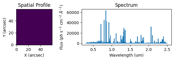
NOTE Plotting results for higher values of R takes forever because the array size gets pretty large
Extragalactic transient: Supernova
Template spectra can be pulled from A-star Vienna’s spextra package library: https://scopesim.univie.ac.at/spextra/database/libraries/
from spextra import Spextrum
sed = Spextrum('brown/NGC3870')
[23]:
# base galaxy
gal = sim_tp.galaxy(sed='brown/NGC3870', z=0.02, amplitude=15, filter_curve='g', pixel_scale=1, r_eff=2.5, n=1., ellip=0.3, theta=0, extend=5)
plot_source(gal)

# download spectrum from spextra library
from spextra import Spextrum
sed = Spextrum('sne/sn1a').redshift(0.02) # redshift it to match the host galaxy
spec = sed.scale_to_magnitude(14*u.ABmag, 'g')
spec.plot()
# add sn to gal at 5",5" offset from center
gal.append(Source(spectra=spec, x=[5.0], y=[5.0], ref=[0.], weight=[1.0]))


[22]:
im = gal.image(wave_min=0.3, wave_max=2.5, pixel_scale=1*u.arcsec)
im.plot()
astar.scopesim.optics.image_plane - No BUNIT found in added HDU.
py.warnings - WARNING: /Users/yashvi/Desktop/ZShooter/ScopeSim/scopesim/source/source.py:501: DeprecationWarning: Adding a table directly to the ImagePlane is deprecated since v0.10.0. Passing a table to ImagePlane.add() will raise an error from version 0.12 onwards. Use FOV to add tables and image HDUs together before.
  im_plane.add(hdu_or_table, sub_pixel=sub_pixel,
[22]:
(<Figure size 640x480 with 2 Axes>, <Axes: >)
